import numpy as np
import pandas as pd
from sklearn import decomposition
from pymongo import MongoClient 
from sklearn.pipeline import Pipeline
from sklearn.impute import KNNImputer
from sklearn.base import BaseEstimator, TransformerMixin
from sklearn.preprocessing import StandardScaler
from sklearn.compose import ColumnTransformer
from scipy import stats
from sklearn.preprocessing import PowerTransformer
import numpy as np
from sklearn.manifold import Isomap
import matplotlib.pyplot as plt
from sklearn.metrics import  mean_absolute_percentage_error
import pandas as pd
from sklearn.preprocessing import LabelEncoder
from sklearn.model_selection import StratifiedShuffleSplit
from sklearn.preprocessing import PowerTransformer
# To use this experimental feature, we need to explicitly ask for it:
from sklearn.experimental import enable_iterative_imputer  # noqa
from sklearn.datasets import fetch_california_housing
from sklearn.impute import SimpleImputer
from sklearn.impute import IterativeImputer
from sklearn.linear_model import BayesianRidge
from sklearn.tree import DecisionTreeRegressor
from sklearn.ensemble import ExtraTreesRegressor
from sklearn.neighbors import KNeighborsRegressor
from sklearn.pipeline import make_pipeline
from sklearn.model_selection import cross_val_score
import plotly.graph_objects as go
import plotly.tools as tls
from plotly.offline import plot, iplot, init_notebook_mode
from IPython.core.display import display, HTML
from plotly.subplots import make_subplots
from sklearn.model_selection import GridSearchCV
from sklearn.decomposition import TruncatedSVD
from xgboost.sklearn import XGBRegressor
from sklearn.ensemble import RandomForestRegressor
from sklearn.model_selection import cross_val_score
init_notebook_mode(connected = True)
config={'showLink': False, 'displayModeBar': False}

num_att = ['First Registration',
 'Mileage',
 'Power(hp)',
 'Displacement']

X_num_att = ['First Registration',
 'Mileage',
 'Power(hp)',
 'Displacement']

cat_att = ['Make', 'Model', 'Body', 'Fuel','Gearing Type']


class InitalCleaning(BaseEstimator, TransformerMixin):
    def __init__(self):
        pass
    def fit(self, X, y=None):
        return self
    def transform(self, play_df, y = None):
        play_df = play_df.drop(columns = ['ID', 'Loaded_in_DW', 'Model Code'])
        
        #Adjust Column Types
        play_df['Power(hp)'] = pd.to_numeric(play_df['Power(hp)'])
        play_df['Displacement'] = pd.to_numeric(play_df['Displacement'])
        play_df['Mileage'] = pd.to_numeric(play_df['Mileage'])
        play_df['Price'] = pd.to_numeric(play_df['Price'])
        
        #Drop rows with null values
        play_df = play_df[~(play_df['Make'].isna() | play_df['Model'].isna())]
        play_df = play_df[~(play_df['Displacement'].isna() & play_df['Power(hp)'].isna())]
        play_df = play_df[~(play_df["Body"].isna())]
        play_df = play_df[~(play_df["Fuel"].isna())]
        play_df = play_df[~(play_df["Price"].isna())]
        
        #Drop fake ads and update column values
        play_df = play_df[~(play_df['Displacement'] < 900)]
        play_df = play_df[~(play_df['Displacement'] > 70000)]
        play_df = play_df[~((play_df['Power(hp)']>500) & \
                        (~((play_df['Make'] == 'Audi') | (play_df['Make'] == 'BMW')  | (play_df['Make'] == 'Mercedes-Benz'))))]
        play_df = play_df[~((play_df['Power(hp)']<30) & (~(play_df['Fuel'] == 'Electricity')))]
        play_df = play_df[~(play_df['Price']>300000)]
        play_df["Fuel"] = play_df["Fuel"].str.split("/").str[0]
        play_df['Gearing Type'] = play_df['Gearing Type'].replace({np.nan : 'Manual'})

        
        return play_df
    
    
class AdjustEquip(BaseEstimator, TransformerMixin):
    def __init__(self):
        pass
    def fit(self, X, y=None):
        return self
    def transform(self, play_df, y = None):
        #Keep only 0 and 1 values
        equipment = play_df.iloc[:,9:79]
        equipment = equipment.replace({np.nan: 0})
        equipment = equipment.replace({'1': 1})
        a = set(equipment['Warranty'])
        a.remove(0)
        a.remove(1)
        equipment = equipment.replace(list(a) , 1)
        
        #Convert each column's type to int
        for col in equipment.columns:
            equipment[col] = equipment[col].astype(int)
        play_df.iloc[:,9:79] = equipment

        
        return play_df
    
class CategoricalEncoder(BaseEstimator, TransformerMixin):
    def __init__(self):
        pass
    def fit(self, X, y=None):
        return self
    def transform(self, play_df, y = None):
        
        play_df = pd.get_dummies(data = play_df,
                                      columns = ['Make', 'Model', 'Body', 'Fuel','Gearing Type'],
                                      dummy_na = False)
        
        
        return play_df

class RegistrationTransformer(BaseEstimator, TransformerMixin):
    def __init__(self, tip = 0):
        self.tip = tip
    def fit(self, X, y=None):
        return self
    def transform(self, play_df, y = None):
        
        #Reset index is used to avoid null values when merging
        play_df.reset_index(drop=True, inplace=True)
        a = date_magic(play_df['First Registration'])
        a.reset_index(drop = True, inplace = True)
        play_df['First Registration'] = a
        
        if self.tip == 0:
             play_df = play_df[(play_df['Make']=='BMW') & (play_df['First Registration'] > 2005) & ( (play_df['Model'].str.startswith('3')) | (play_df['Model'].str.startswith('1'))  ) ]
        elif self.tip == 1:
             play_df = play_df[play_df.isnull().any(axis=1)] 
        return play_df


class IQROutlierRemoval_new(BaseEstimator, TransformerMixin):
    def __init__(self, num_att):
        self.num_att = num_att
    def fit(self, X, y = None):
        return self
    def transform(self, play_df, y = None):
         
#         Q1 = play_df.quantile(0.25)
#         Q3 = play_df.quantile(0.75)
#         IQR = Q3- Q1
#         play_df = play_df[~((play_df < (Q1 - 1.5 * IQR)) |(play_df > (Q3 + 1.5 * IQR))).any(axis=1)]
        return pd.DataFrame(play_df, columns = num_att)


class IQROutlierRemoval(BaseEstimator, TransformerMixin):
    def __init__(self, num_att):
        self.num_att = num_att
    def fit(self, X, y = None):
        return self
    def transform(self, play_df, y = None):
        bmw_num = play_df[self.num_att]
        bmw_cat = play_df.drop(self.num_att, axis = 1)
        Q1 = bmw_num.quantile(0.25)
        Q3 = bmw_num.quantile(0.75)
        IQR = Q3- Q1
        bmw_num = bmw_num[~((bmw_num < (Q1 - 1.5 * IQR)) |(bmw_num > (Q3 + 1.5 * IQR))).any(axis=1)]
        return pd.DataFrame(bmw_num, columns = num_att)
    

class ZScoreOutlierRemoval(BaseEstimator, TransformerMixin):
    def __init__(self, num_att):
        self.num_att = num_att
    def fit(self, X, y = None):
        return self
    def transform(self, play_df, y = None):
        z = np.abs(stats.zscore(play_df, nan_policy='omit'))
        return play_df[(z < 3).all(axis=1)]
    

class StandardScalerIndices(BaseEstimator, TransformerMixin):
    def __init__(self):
        self.scaler = StandardScaler()
    def fit(self, X, y=None):
        self.scaler.fit(X)
        return self
    def transform(self, play_df, y = None):     
        return pd.DataFrame(self.scaler.transform(play_df),columns = play_df.columns, index = play_df.index)

    
class PowerTransformerIndices(BaseEstimator, TransformerMixin):
    def __init__(self, method):
        self.method = method
        self.transformer = PowerTransformer(method = self.method)
    def fit(self, X, y=None):
        self.transformer.fit(X)
        return self
    def transform(self, play_df, y = None):
        return pd.DataFrame(self.transformer.transform(play_df),columns = play_df.columns, index = play_df.index)
    
    
class RemovePrice(BaseEstimator, TransformerMixin):
    def __init__(self):
        pass
    def fit(self, X, y = None):
        return self
    def transform(self, play_df, y = None):
        return play_df.drop('Price', axis = 1)

class IterativeImputerIndices(BaseEstimator, TransformerMixin):
    def __init__(self, estimator):
        self.imputer = IterativeImputer(estimator = estimator)
    def fit(self, X, y=None):
        self.imputer.fit(X)
        return self
    def transform(self, play_df, y = None):
        return pd.DataFrame(self.imputer.transform(play_df),columns = play_df.columns, index = play_df.index)

class JoinTransformer(BaseEstimator, TransformerMixin):
    def __init__(self, BMW_df, new_att):
        self.BMW_df = BMW_df
        self.new_att = new_att
    def fit(self,X,y = None):
        return self
    def transform(self, X, y = None):
        new = self.BMW_df.drop(self.new_att, axis = 1)
        return X.join(new)
        

def date_magic(d):
    months_dict = {'Jan': 1,'Feb':2,'Mar':3,'Apr':4 ,'May':5 ,'Jun':6,'Jul':7,
                      'Aug':8,'Sep':9,'Oct':10 ,'Nov':11,'Dec':12}
    year = []
    month = []
    num_year = []
    for el in d:
        el = str(el)

        split = el.split('-')
        if (len(split)>1):
            month.append(months_dict[split[0]])
            if(int(split[1])>20):
                year.append(int('19' + split[1]))
            else:
                year.append(int('20' + split[1]))
            continue

        split = el.split('/')
        if(len(split)>1):
            month.append(int(split[0]))
            year.append(int(split[1]))
            continue

        month.append(1)
        year.append(int(el))
    month = pd.Series(month)
    year  = pd.Series(year)
    num_year = year + month/12  
    return pd.Series(num_year)


def readData():

    client = MongoClient('mongodb+srv://<User>:<Pass>@dwprojectcluster.lpqbf.mongodb.net/cars_database?retryWrites=true&w=majority')

    df_cars = pd.DataFrame(list(client.cars_database.cars.find({})))
    df_cars.drop('_id', axis = 1, inplace = True)
    df_cars = df_cars[df_cars['Loaded_in_DW'].eq(False)]
    df_cars.drop_duplicates(subset=['ID'], inplace = True)
    
    return df_cars




recnik = {}
recnik['Method'] = []
recnik['Mean Percentage Error'] = []
recnik['Standard Deviation'] = []
def randomforestCV( max_features, n_estimators, X, y, message, scoring = 'neg_mean_absolute_percentage_error', recnik = recnik):
    rfr = RandomForestRegressor(max_features = max_features, n_estimators = n_estimators, random_state = 2)
    rfr.fit(X,y)
    rfr_scores = cross_val_score(rfr, X, y, scoring = scoring, cv = 5, n_jobs = -1)
    print("Scores:", -rfr_scores)
    print("Mean:", -rfr_scores.mean())
    print("Standard deviation:", rfr_scores.std())
    recnik['Method'].append(message)
    recnik['Mean Percentage Error'].append(-rfr_scores.mean())
    recnik['Standard Deviation'].append(rfr_scores.std())

    
def gridSearch(param_grid, model, X, y):
    grid_search = GridSearchCV(model, param_grid, cv=5,
                           scoring='neg_mean_absolute_percentage_error',
                           return_train_score=True,
                           verbose = 10, n_jobs = -1)
    grid_search.fit(X, y)
    cvres = grid_search.cv_results_
    for mean_score, params in zip(cvres["mean_test_score"], cvres["params"]):
        print(-mean_score, params)
    return grid_search

df_cars = readData()
type0_pipeline = Pipeline([
                        ('initial', InitalCleaning()),
                        ('equipment', AdjustEquip()),
                        ('date', RegistrationTransformer(tip = 0))
                    ])

type1_pipeline = Pipeline([
                        ('initial', InitalCleaning()),
                        ('equipment', AdjustEquip()),
                        ('date', RegistrationTransformer(tip = 1)),
                        ('encoder', CategoricalEncoder())
                    ])

no_category = Pipeline([
                        ('initial', InitalCleaning()),
                        ('equipment', AdjustEquip()),
                        ('date', RegistrationTransformer(tip = 0)),
                    ])


BMW_df = type0_pipeline.fit_transform(df_cars)
nan_df = type1_pipeline.fit_transform(df_cars)
viz_df = no_category.fit_transform(df_cars)

BMW_df = BMW_df.reset_index()
BMW_df = BMW_df.drop('index', axis = 1)
split = StratifiedShuffleSplit(n_splits=1, test_size=0.01, random_state=42)
for train_index, test_index in split.split(BMW_df, BMW_df["Model"]):
    strat_train_set = BMW_df.loc[train_index]
    strat_test_set = BMW_df.loc[test_index]

y_train = strat_train_set['Price']
x_train = strat_train_set.drop('Price', axis = 1)
y_test = strat_test_set['Price']
x_test = strat_test_set.drop('Price', axis = 1)

import pandas_profiling as pp

from plotly.offline import plot, iplot, init_notebook_mode
from IPython.core.display import display, HTML
init_notebook_mode(connected = True)
config={'showLink': False, 'displayModeBar': False}


pp.ProfileReport(viz_df.iloc[:,np.r_[0:10]]).to_file('aa.html')

N_SPLITS = 5

rng = np.random.RandomState(0)
X = nan_df.drop(columns = ['Price'])
y = nan_df['Price']
X = X.to_numpy()
y = y.to_numpy()
score_simple_imputer = pd.DataFrame()
br_estimator = BayesianRidge()
for strategy in ('mean', 'median'):
    estimator = make_pipeline(
        SimpleImputer(missing_values=np.nan, strategy=strategy),
        br_estimator
    )
    score_simple_imputer[strategy] = cross_val_score(
        estimator, X, y, scoring='neg_mean_squared_error',
        cv=N_SPLITS
    )
score_simple_imputer

X = X[::5]
y = y[::5]
estimators = [
    DecisionTreeRegressor(max_features='sqrt', random_state=0),
    ExtraTreesRegressor(n_estimators=10, random_state=0),
    KNeighborsRegressor(n_neighbors=15),
    BayesianRidge()
]
score_iterative_imputer = pd.DataFrame()
for impute_estimator in estimators:
    estimator = make_pipeline(
        IterativeImputer(random_state=0, estimator=impute_estimator),
        br_estimator
    )
    
    score_iterative_imputer[impute_estimator.__class__.__name__] = \
        cross_val_score(
            estimator, X, y, scoring='neg_mean_squared_error', verbose = 2,
            cv=N_SPLITS
        )
score_iterative_imputer
;

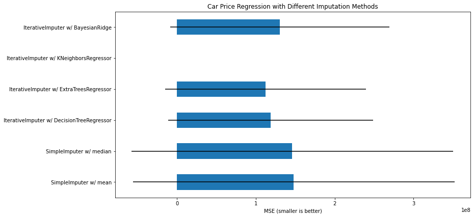
scores = pd.concat(
    [score_simple_imputer, score_iterative_imputer],
    keys=['SimpleImputer', 'IterativeImputer'], axis=1
)

# plot california housing results
fig, ax = plt.subplots(figsize=(13, 6))
means = -scores.mean()
errors = scores.std()
means.plot.barh(xerr=errors, ax=ax)
ax.set_title('Car Price Regression with Different Imputation Methods')
ax.set_xlabel('MSE (smaller is better)')
ax.set_yticks(np.arange(means.shape[0]))
ax.set_yticklabels([" w/ ".join(label) for label in means.index.tolist()])
plt.tight_layout(pad=1)
plt.show()

from sklearn.preprocessing import PowerTransformer

final_pipeline = Pipeline([
                        ('IQR_removal',IQROutlierRemoval(num_att = num_att)),
                        ('std_scaler', StandardScalerIndices()),
                        ('yeo-johnson',PowerTransformerIndices(method='yeo-johnson')),
                        ('z_score_removal', ZScoreOutlierRemoval(num_att = num_att)),
                        ('Imputer', IterativeImputerIndices(estimator = ExtraTreesRegressor(n_estimators=10, random_state=0))),
                        ('join', JoinTransformer(x_train, num_att)), #kategoriski so numericki
                        ('encoder', CategoricalEncoder()),
                        

                        ])


X_train_prepared = pd.DataFrame(final_pipeline.fit_transform(x_train))

joined = X_train_prepared.join(y_train)
y_train = joined['Price']

fig = go.Figure()


fig.add_trace(
    go.Histogram(x=X_train_prepared['Mileage'], name='Mileage', visible = True)
)
fig.add_trace(
    go.Histogram(x=X_train_prepared['First Registration'], name='First Registration', visible = False)
)
fig.add_trace(
    go.Histogram(x=X_train_prepared['Power(hp)'], name='Power(hp)', visible = False)
)
fig.add_trace(
    go.Histogram(x=X_train_prepared['Displacement'], name='Displacement', visible = False)
)
fig.update_layout(
    updatemenus=[
        dict(
            active=0,
            buttons=list([
                dict(label="Mileage",
                     method="update",
                     args=[{"visible": [True,False,False,False]},
                           {"title": "Mileage"
                            }]),
                dict(label="First Registration",
                     method="update",
                     args=[{"visible": [False,True,False,False]},
                           {"title": "First Registration"}]),
                dict(label="Power(hp)",
                     method="update",
                     args=[{"visible": [False,False,True,False]},
                           {"title": "Power(hp)"}]),
                dict(label="Displacement",
                     method="update",
                     args=[{"visible": [False,False,False,True]},
                           {"title": "Displacement"}]),
               
            ]),
                       
        )
    ])

plot(fig, filename = 'fig.html', config = config)
display(HTML('fig.html'))

pca = decomposition.PCA()
pca.n_components = 121
pca_data = pca.fit_transform(X_train_prepared)
percentage_var_explained = pca.explained_variance_ / np.sum(pca.explained_variance_)
cum_var_explained = np.cumsum(percentage_var_explained)

svd = TruncatedSVD()
svd.n_components = 121
svd_data = svd.fit_transform(X_train_prepared)
percentage_var_explained_svd = svd.explained_variance_ / np.sum(svd.explained_variance_)
cum_var_explained_svd = np.cumsum(percentage_var_explained_svd)


fig = go.Figure()
fig.add_trace(go.Scatter(y = cum_var_explained,  name = 'PCA'))
fig.add_trace(go.Scatter(y = cum_var_explained_svd,  name = 'SVD'))

fig.update_layout(plot_bgcolor='rgb(255,255,255)',xaxis_title="n_components",
    yaxis_title='Variance')
fig.update_xaxes(ticks = 'outside', showline=True, linecolor='black')
fig.update_yaxes(ticks = 'outside', showline=True, linecolor='black')

# Plot figure
plot(fig, filename = 'fig2.html', config = config)
display(HTML('fig2.html'))

pca_pipeline = Pipeline([
                        ('IQR_removal',IQROutlierRemoval(num_att = num_att)),
                        ('std_scaler', StandardScalerIndices()),
                        ('yeo-johnson',PowerTransformerIndices(method='yeo-johnson')),
                        ('z_score_removal', ZScoreOutlierRemoval(num_att = num_att)),
                        ('Imputer', IterativeImputerIndices(estimator = ExtraTreesRegressor(n_estimators=10, random_state=0))),
                        ('join', JoinTransformer(x_train, num_att)), #kategoriski so numericki
                        ('encoder', CategoricalEncoder()),
                        ('pca', decomposition.PCA(n_components = 86))
                        ])

spca_pipeline = Pipeline([
                        ('IQR_removal',IQROutlierRemoval(num_att = num_att)),
                        ('std_scaler', StandardScalerIndices()),
                        ('yeo-johnson',PowerTransformerIndices(method='yeo-johnson')),
                        ('z_score_removal', ZScoreOutlierRemoval(num_att = num_att)),
                        ('Imputer', IterativeImputerIndices(estimator = ExtraTreesRegressor(n_estimators=10, random_state=0))),
                        ('join', JoinTransformer(x_train, num_att)), #kategoriski so numericki
                        ('encoder', CategoricalEncoder()),
                        ('pca', decomposition.SparsePCA())
                        ])

svd_pipeline = Pipeline([
                        ('IQR_removal',IQROutlierRemoval(num_att = num_att)),
                        ('std_scaler', StandardScalerIndices()),
                        ('yeo-johnson',PowerTransformerIndices(method='yeo-johnson')),
                        ('z_score_removal', ZScoreOutlierRemoval(num_att = num_att)),
                        ('Imputer', IterativeImputerIndices(estimator = ExtraTreesRegressor(n_estimators=10, random_state=0))),
                        ('join', JoinTransformer(x_train, num_att)), #kategoriski so numericki
                        ('encoder', CategoricalEncoder()),
                        ('svd', TruncatedSVD(n_components = 86))
                        ])

isomap_pipeline = Pipeline([
                        ('IQR_removal',IQROutlierRemoval(num_att = num_att)),
                        ('std_scaler', StandardScalerIndices()),
                        ('yeo-johnson',PowerTransformerIndices(method='yeo-johnson')),
                        ('z_score_removal', ZScoreOutlierRemoval(num_att = num_att)),
                        ('Imputer', IterativeImputerIndices(estimator = ExtraTreesRegressor(n_estimators=10, random_state=0))),
                        ('join', JoinTransformer(x_train, num_att)), #kategoriski so numericki
                        ('encoder', CategoricalEncoder()),
                        ('isomap', Isomap(n_components = 60))
                        ])

X_train_spca = pd.DataFrame(spca_pipeline.fit_transform(x_train))
X_train_pca = pd.DataFrame(pca_pipeline.fit_transform(x_train))
y_train_pca = y_train.reset_index()
y_train_pca = y_train_pca.drop('index', axis = 1)

X_train_svd = pd.DataFrame(svd_pipeline.fit_transform(x_train))
y_train_svd = y_train_pca.copy()

X_train_isomap = pd.DataFrame(isomap_pipeline.fit_transform(x_train))
y_train_isomap = y_train_pca.copy()
;

safety = ['ABS','Traction control','Driver-side airbag','Side airbag','Passenger-side airbag','Isofix','Immobilizer']
luxury = ['Adaptive Cruise Control','Leather steering wheel','Massage seats','Heated steering wheel','Panorama roof','Touch screen',
          'Keyless central door lock','Electrically heated windshield','Alloy wheels','Sunroof','Electrically adjustable seats',
         'Navigation system']
general = ['Multi-function steering wheel','Air suspension','Hill Holder','USB','Non-smoking Vehicle','Air conditioning','Automatic climate control','Radio','Bluetooth', 'CD player',
          'Power windows','Central door lock','On-board computer','Alarm system', 'Trailer hitch', 'Ski bag','MP3','Digital radio',
          'Armrest','Power steering','Electrical side mirrors','Roof rack']
sensors = ['Parking assist system sensors rear','Parking assist system sensors front','Night view assist', 'Blind spot monitor',  'Parking assist system camera'
          , 'Parking assist system self-steering','Lane departure warning system','Traffic sign recognition',
           'Electronic stability control','Tire pressure monitoring system','Electric tailgate','Rain sensor','Start-stop system']
lights = ['LED Daytime Running Lights','LED Headlights','Adaptive headlights','Daytime running lights','Xenon headlights','Fog lights']
recnik2 = {'luxury':luxury, 'safety':safety, 'general':general, 'sensors':sensors, 'lights':lights}




num_att_new = ['First Registration',
 'Mileage',
 'Power(hp)',
 'Displacement', 'luxury', 'safety', 'general', 'lights', 'sensors']
x_train_red = x_train.copy()
for key in recnik2.keys():
    x_train_red
    x_train_red[key] = 0
    for obj in recnik2[key]:
        x_train_red[key] += x_train_red[obj]
        x_train_red = x_train_red.drop(obj, axis = 1)

        

spca_pipeline_reduced = Pipeline([
                        ('IQR_removal',IQROutlierRemoval(num_att = num_att_new)),
                        ('std_scaler', StandardScalerIndices()),
                        ('yeo-johnson',PowerTransformerIndices(method='yeo-johnson')),
                        ('z_score_removal', ZScoreOutlierRemoval(num_att = num_att_new)),
                        ('Imputer', IterativeImputerIndices(estimator = ExtraTreesRegressor(n_estimators=10, random_state=0))),
                        ('join', JoinTransformer(x_train_red, num_att_new)), #kategoriski so numericki
                        ('encoder', CategoricalEncoder()),
                        #('pca', decomposition.SparsePCA())
                        ])


reduced_x = pd.DataFrame(spca_pipeline_reduced.fit_transform(x_train_red))
joined = reduced_x.join(y_train)
reduced_y = joined['Price']
reduced_reset_y = reduced_y.reset_index()
reduced_reset_y = reduced_reset_y.drop('index', axis = 1 )

;

svd = TruncatedSVD()
svd.n_components = 60
svd_data = svd.fit_transform(reduced_x,reduced_y)
percentage_var_explained_svd = svd.explained_variance_ / np.sum(svd.explained_variance_)
cum_var_explained_svd = np.cumsum(percentage_var_explained_svd)

pca = decomposition.PCA()
pca.n_components = 60
pca_data = pca.fit_transform(reduced_x,reduced_y)
percentage_var_explained = pca.explained_variance_ / np.sum(pca.explained_variance_)
cum_var_explained = np.cumsum(percentage_var_explained)



fig = go.Figure()
fig.add_trace(go.Scatter(y = cum_var_explained,  name = 'PCA'))
fig.add_trace(go.Scatter(y = cum_var_explained_svd,  name = 'SVD'))

fig.update_layout(plot_bgcolor='rgb(255,255,255)',xaxis_title="n_components",
    yaxis_title='Variance')
fig.update_xaxes(ticks = 'outside', showline=True, linecolor='black')
fig.update_yaxes(ticks = 'outside', showline=True, linecolor='black')

# Plot figure
plot(fig, filename = 'fig10.html', config = config)
display(HTML('fig10.html'))

spca_pipeline_reduced2 = Pipeline([
                        ('IQR_removal',IQROutlierRemoval(num_att = num_att_new)),
                        ('std_scaler', StandardScalerIndices()),
                        ('yeo-johnson',PowerTransformerIndices(method='yeo-johnson')),
                        ('z_score_removal', ZScoreOutlierRemoval(num_att = num_att_new)),
                        ('Imputer', IterativeImputerIndices(estimator = ExtraTreesRegressor(n_estimators=10, random_state=0))),
                        ('join', JoinTransformer(x_train_red, num_att_new)), #kategoriski so numericki
                        ('encoder', CategoricalEncoder()),
                        ('pca', decomposition.SparsePCA())
                        ])

pca_pipeline_reduced = Pipeline([
                        ('IQR_removal',IQROutlierRemoval(num_att = num_att_new)),
                        ('std_scaler', StandardScalerIndices()),
                        ('yeo-johnson',PowerTransformerIndices(method='yeo-johnson')),
                        ('z_score_removal', ZScoreOutlierRemoval(num_att = num_att_new)),
                        ('Imputer', IterativeImputerIndices(estimator = ExtraTreesRegressor(n_estimators=10, random_state=0))),
                        ('join', JoinTransformer(x_train_red, num_att_new)), #kategoriski so numericki
                        ('encoder', CategoricalEncoder()),
                        ('pca', decomposition.PCA(n_components = 34))
                        ])


svd_pipeline_reduced = Pipeline([
                        ('IQR_removal',IQROutlierRemoval(num_att = num_att_new)),
                        ('std_scaler', StandardScalerIndices()),
                        ('yeo-johnson',PowerTransformerIndices(method='yeo-johnson')),
                        ('z_score_removal', ZScoreOutlierRemoval(num_att = num_att_new)),
                        ('Imputer', IterativeImputerIndices(estimator = ExtraTreesRegressor(n_estimators=10, random_state=0))),
                        ('join', JoinTransformer(x_train_red, num_att_new)), #kategoriski so numericki
                        ('encoder', CategoricalEncoder()),
                        ('SVD', TruncatedSVD(n_components = 34))
                        ])
reduced_x_spca = pd.DataFrame(spca_pipeline_reduced2.fit_transform(x_train_red))
reduced_x_svd = pd.DataFrame(svd_pipeline_reduced.fit_transform(x_train_red))
reduced_x_pca = pd.DataFrame(pca_pipeline_reduced.fit_transform(x_train_red))

final_pipeline = Pipeline([
                        ('IQR_removal',IQROutlierRemoval(num_att = num_att)),
                        ('std_scaler', StandardScalerIndices()),
                        ('yeo-johnson',PowerTransformerIndices(method='yeo-johnson')),
                        ('z_score_removal', ZScoreOutlierRemoval(num_att = num_att)),
                        ('Imputer', IterativeImputerIndices(estimator = ExtraTreesRegressor(n_estimators=10, random_state=0))),
                        ('join', JoinTransformer(x_train, num_att)), #kategoriski so numericki
                        
                        

                        ])


X_train_label = pd.DataFrame(final_pipeline.fit_transform(x_train))


cat = [ 'Make','Model', 'Fuel', 'Body', 'Gearing Type']
encoder = LabelEncoder()
for c in cat:
    X_train_label[c] = encoder.fit_transform(X_train_label[c])

spca = decomposition.SparsePCA()
X_train_label_sparse = pd.DataFrame(spca.fit_transform(X_train_label)) 

grid_no_dim_red = gridSearch(param_grid = {'max_features' : [90,100,110,'auto','sqrt','log2'], 'n_estimators' : [100] }, 
                             model = RandomForestRegressor(random_state = 2), X = X_train_prepared, y = y_train)
randomforestCV(max_features = grid_no_dim_red.best_params_['max_features'], n_estimators = grid_no_dim_red.best_params_['n_estimators'],
               X = X_train_prepared, y = y_train, message = 'Without dim reduction')

grid_pca = gridSearch(param_grid = {'n_estimators':[100], 'max_features' : [50,60,70,'auto', 'sqrt', 'log2']}, 
                             model = RandomForestRegressor(random_state =2), X = X_train_pca, y = y_train_pca)
randomforestCV(max_features = grid_pca.best_params_['max_features'], 
               n_estimators = grid_pca.best_params_['n_estimators'],
               X = X_train_pca, y = y_train_pca, message = 'PCA applied')

grid_spca = gridSearch(param_grid = {'n_estimators':[100], 'max_features' : [50,60,70,80, 'auto','sqrt','log2']}, 
                             model = RandomForestRegressor(random_state =2), X = X_train_spca, y = y_train_pca)
randomforestCV(max_features = grid_spca.best_params_['max_features'], 
               n_estimators = grid_spca.best_params_['n_estimators'],
               X = X_train_spca, y = y_train_pca, message = 'SparsePCA applied')

grid_svd = gridSearch(param_grid = {'n_estimators':[100], 'max_features' : [40,50,60,70, 'auto','sqrt','log2']}, 
                             model = RandomForestRegressor(random_state = 2), X = X_train_svd, y = y_train_svd.values.ravel())
randomforestCV(max_features = grid_svd.best_params_['max_features'], 
               n_estimators = grid_svd.best_params_['n_estimators'],
               X = X_train_svd, y = y_train_svd.values.ravel(), message = 'SVD applied')

grid_reduced = gridSearch(param_grid = {'n_estimators':[100], 'max_features' : [15,20,25,30,40,50,'auto','sqrt','log2']}, 
                             model = RandomForestRegressor(random_state =2), X = reduced_x, y = reduced_y)
randomforestCV(max_features = grid_reduced.best_params_['max_features'], 
               n_estimators = grid_reduced.best_params_['n_estimators'],
                X = reduced_x, y = reduced_y, message = 'Reduced Data Set w/o dim reduction')

grid_reduced_PCA = gridSearch(param_grid = {'n_estimators':[100], 'max_features' : [10,15,20,25,30,'auto','sqrt','log2']}, 
                             model = RandomForestRegressor(random_state = 2), X = reduced_x_pca, y = reduced_reset_y.values.ravel())
randomforestCV(max_features = grid_reduced_PCA.best_params_['max_features'], 
               n_estimators = grid_reduced_PCA.best_params_['n_estimators'],
                X = reduced_x_pca, y = reduced_reset_y.values.ravel(), message = 'Reduced Data Set + PCA')

grid_reduced_SPCA = gridSearch(param_grid = {'n_estimators':[100], 'max_features' : [10,15,20,21,'auto','sqrt','log2',40]}, 
                             model = RandomForestRegressor(random_state = 2), X = reduced_x_spca, y = reduced_reset_y.values.ravel())
randomforestCV(max_features = grid_reduced_SPCA.best_params_['max_features'], 
               n_estimators = grid_reduced_SPCA.best_params_['n_estimators'],
                X = reduced_x_spca, y = reduced_reset_y.values.ravel(), message = 'Reduced Data Set + SparsePCA')

grid_reduced_svd = gridSearch(param_grid = {'n_estimators':[100], 'max_features' : [10,15,20,25,30,'auto','sqrt','log2']}, 
                             model = RandomForestRegressor(random_state =42), X = reduced_x_svd, y = reduced_reset_y.values.ravel())
randomforestCV(max_features = grid_reduced_svd.best_params_['max_features'], 
               n_estimators = grid_reduced_svd.best_params_['n_estimators'],
                X = reduced_x_svd, y = reduced_reset_y.values.ravel(), message = 'Reduced Data Set + SVD')

rfr = RandomForestRegressor(random_state = 2,max_depth=17)
rfr.fit(X_train_label,y_train)
rfr_scores = cross_val_score(rfr, X_train_label, y_train, scoring = 'neg_mean_absolute_percentage_error', 
                             cv = 5, n_jobs = -1)
recnik['Method'].append('Label Encoded w/o Dimenisonality Reduction')
recnik['Mean Percentage Error'].append(-rfr_scores.mean())
recnik['Standard Deviation'].append(rfr_scores.std())

xgb = XGBRegressor(random_state = 2) 
xgb.fit(X_train_prepared, y_train)
xgb_scores = cross_val_score(xgb, X_train_prepared, y_train, scoring = 'neg_mean_absolute_percentage_error', cv = 5, n_jobs = -1)

print("Scores:", -xgb_scores)
print("Mean:", -xgb_scores.mean())
print("Standard deviation:", xgb_scores.std())
recnik['Method'].append('XGBRegressor w/o dim reduction')
recnik['Mean Percentage Error'].append(-xgb_scores.mean())
recnik['Standard Deviation'].append(xgb_scores.std())

from sklearn.ensemble import VotingRegressor

vote_mod = VotingRegressor([ ('XGBRegressor', XGBRegressor()), 
                            ('RandomForest', RandomForestRegressor(random_state = 2,max_depth=17))])
vote_mod.fit(X_train_label, y_train)
reg_scores = cross_val_score(vote_mod, X_train_label, y_train, scoring = 'neg_mean_absolute_percentage_error', 
                             cv = 5, n_jobs = -1)


print("Scores:", -reg_scores)
print("Mean:", -reg_scores.mean())
print("Standard deviation:", reg_scores.std())

recnik['Method'].append('Voting Regressor w/o dim reduction')
recnik['Mean Percentage Error'].append(-reg_scores.mean())
recnik['Standard Deviation'].append(reg_scores.std())

reg_scores = cross_val_score(vote_mod, X_train_label_sparse, y_train_pca.values.ravel(), scoring = 'neg_mean_absolute_percentage_error', 
                             cv = 5)
print("Scores:", -reg_scores)
print("Mean:", -reg_scores.mean())
print("Standard deviation:", reg_scores.std())

recnik['Method'].append('Voting Regressor + SparsePCA')
recnik['Mean Percentage Error'].append(-reg_scores.mean())
recnik['Standard Deviation'].append(reg_scores.std())

pd.DataFrame.from_dict(recnik)